Optimizing LSTM's on GPU with scheduling
Summary
In the Optim-LSTM project, we aim to produce a high-performance implementation of Long-Short Term Memory Network using Domain-Specific Languages such as Halide and/or using custom DSL. This would provide portability across different platforms and architectures.
Background
LSTM’s are a variant of RNN and were designed to tackle the vanishing gradients problem with RNN. RNN’s when back-propogated over a large number of time-steps, face a problem of diminished value of gradients. With the presence of memory cell in LSTM’s, we can have continuous gradient flow which helps in learning long-term dependencies. Equations describing LSTM network:
\[i\_{t} = sigm(\theta\_{xi} X\_{t} + \theta\_{hi} h\_{t-1} + b\_{i})\] \[f\_{t} = sigm(\theta\_{xf} X\_{t} + \theta\_{hf} h\_{t-1} + b\_{f})\] \[o\_{t} = sigm(\theta\_{xo} X\_{t} + \theta\_{ho} h\_{t-1} + b\_{o})\] \[g_{t} = sigm(\theta\_{xg} X\_{t} + \theta\_{hg} h\_{t-1} + b\_{g})\] \[c_{t} = f\_{t} \cdot c\_{t-1} + i\_{t} \cdot g\_{t}\] \[h_{t} = o\_{t} \cdot tanh(c\_{t-1})\]The cost involved in evaluating these networks is dominated by Matrix Matrix Multiplication operation, GEMM operation in BLAS libraries. A naive implementation would perform eight matrix-matrix multiplications, 4 with inputs and 4 with previous state vectors. We plan to explore various optimizations around the naive implementation such as Combining Operations, Fusing Point Wise operations etc.
We plan to initially get familiar with Halide and understand more in depth about Domain Specific Languages and understand the limitations of Halide in tasks not meant for Image Processing such as LSTM’s. Based on our learning and as mentioned in suggested projects, we plan to implement a custom DSL to incorporate variants of RNN’s in the framework. Using the DSL, we aim to use basic blocks from cuDNN or cuBLAS for effecient operations on matrices.
Mid-term checkpoint
We explored the implementation of LSTM using Halide and found that the scheduling policies used in Halide is not optimal/suitable for RNN type neural networks. Instead of starting with DSL implementation, we started working on CUDA implementation of LSTM networks as we think this optimization is key for the goal of term project. Once we have an optimized LSTM kernels, we can link them up with a general purpose framework. We have a generic framework setup in C++ which we can use to call our optimized kernels.
Post Mid-term implementation:
We used the equations as described in Background section to implement the LSTM structure on CUDA. The current baseline version is a naive implementation using cuBLAS library for General purpose matrix multiplication (GEMM). Although GEMM is highly optimized for GPUs, it does not utilize all the parallelism that can be extracted as the matrix sizes are inherently small.
The current implmentation uses 8 GEMM operations, 4 for multiplying input $x_{t}$ with $\theta_{xi},\theta_{xf},\theta_{xo},\theta_{xg}$ and 4 for multiplying $h_{t-1}$ with $\theta_{hi},\theta_{hf},\theta_{ho},\theta_{hg}$.
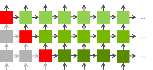 Figure 1: LSTM layer-wise structure
In our current scheduling policy, we first cover the layer l, across the sequence length and then move on to the layer l+1. This implementation does not utilize the inherent parallelism provided by the LSTM structure, but it serves as a valid working baseline.
Below are the key optimizations we are trying to implement.
- Currently our baseline code uses cuBLAS library which does not utilize the complete resource of the GPU and also does not exploit inherent parallelism in LSTM networks. To avoid this problem, we plan to combine multiple matrix multiplications
(Instead of 4 different matrix multiplications). We aim to combine 4 matrix multiplication into one GEMM kernel invocation. This should help in exploiting the available GPU resources. This is due to the usage of all the SM’s on GPU. - As shown in Figure 1, once the computation of first time sequence of first layer
(L0,0)is completed, in our naive implementation we move on to second time step(L0,1)in the same layer. However, since we have the computed output from(L0,0), we can also parallely work on(L1,0)cell. This inherent parallelism increases as we progress through the network and more LSTM cells can be computed in parallel. This scheduling policy is expected to give the most boost in GFLOPS. - Utilizing the FMA units available on the GPU to reduce the number of times a matrix is accessed from memory. For example, we need to perform two matrix multiplcation and one addition to compute $i_{t}, f_{t}, o_{t}, g_{t}$. Instead of storing the intermediate results in a buffer, we plan to compute this in the form of $Y = AX + B$ such that the FMA units are utilized.
Current Runtime
The runtime for our naive implementation of a 4 layer LSTM with below configurations is 182.5ms.
LSTM Config:
- Number of Layers - 4
- Sequence Length - 100
- Hidden Unit Size - 512
- Batch Size - 64
With our proposed optimizations, we expect the runtime to reduce significantly.
Optimizations
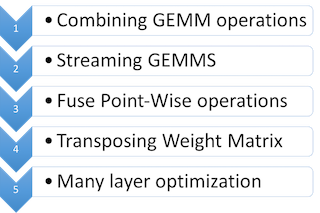
*Figure 2 : Optimizations
As show in Figure 2, we implemented multiple optimizations to optimize the LSTM forward propagation code. We achieve a speedup of 7.98x over the baseline implementation. We have used cuBLAS version 2 in our implimentation to acheive the performance gain.
-
Combining GEMM Operations: In our baseline implementation, we launch matrix multiplications required for LSTM computation individually. We observed that only four of the available SMs were being utilized. Our first goal was to improve the GPU occupancy and increase the resource utilized. In this optimization, we combine multiple smaller matricies and launch a combied matrix multiplication kernel. This utilizes the GPU resources in a much better manner and achieves a speedup of 2x.
-
Streaming GEMMs: There are multiple computations in LSTM which are completely independent of each other. Our baseline code does not exploit this feature and all the computations are done sequentially even if they are independent. Using the Nvidia Stream feature, we can launch multiple kernels which are independent of each other and perform the computation in parallel. With this optimization, we achieve a speedup of 1.82x.
-
Fuse Point-Wise Operations: LSTM computation invloves a lot of point wise operations like tanh, addition and sigmoid. The baseline implementation launches multiple kernels to perform these operations. Launching of multiple kernels in this case is an overhead. We fuse these operations into a single kernel to overcome this inefficiency. With just this optimization, we achieve a speedup of 1.2x. The speedup with this optimization is not significant as compared to the previous speedups. The reason for this is that the amount of point-wise operations is smaller when compared to the overall computations of LSTM.
-
Transposing weight matrix: An obvious optimization to improve the cache locality is to transpose one of the matrix before performing the matrix multiplication. With this optimization, we achieve a speedup of 1.063x. Again, the speedup achieved with only this optimization is not significant. The matrix size is small and multiple operations are not combined into a single GEMM execution. The overhead of performing matrix transpose is high and hence the speedup is less.
-
Many Layer Optimization: As shown in Figure 1, once the computation of first time sequence of first layer
(L0,0)is completed, in our naive implementation we move on to second time step(L0,1)in the same layer. However, since we have the computed output from(L0,0), we can also parallely work on(L1,0)cell. This inherent parallelism increases as we progress through the network and more LSTM cells can be computed in parallel. This scheduling policy is expected to give the most boost in GFLOPS. This optimization helped us achieve a speedup of 1.30x. However, this scheduling algorithm can be used in algorithms for which we have the complete input sequence like in case of sequence to sequence models. However in case of image captioning systems, where the next step input is calculate from the first inputs LSTM output, this scheduling policy is not applicable.
Results
The speedups mentioned in the previous section is for each individual optimization compared to the baseline. We combined multiple combinations of these optimizations and we achieve a speedup of 7.98x overall. The experiments were run with 4 layers of LSTM, each with 100 time sequences, 512 hidden units and 64 batch size.
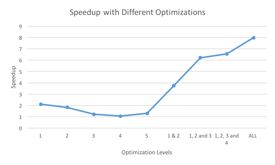 *Figure 3: Speedup with various optimizations
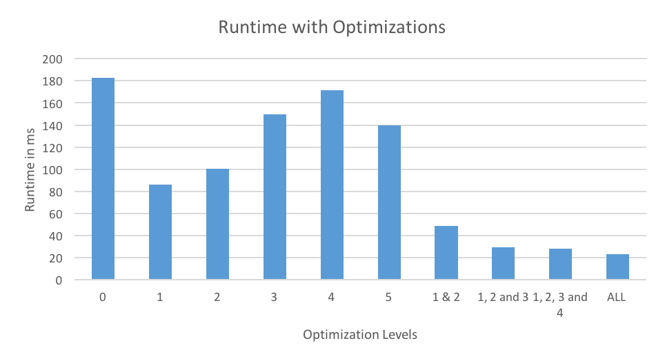 *Figure 4: Runtimes with various optimizations.
Figure 3 and 4 shows the performance of various optimizations with respect to speedup and runtimes. Combining optimizations 1 and 2, we achieve a speedup of 3.74x. In this case, GEMM operations are combined to form a larger matrix and we also use Stream feature to perform independent computations in parallel. By adding the Fuse Point-Wise operations optimization we were able to achieve a further increase in speedup to 6.21x. As explained in the previous section, optimization 4 did not result in any speedup. However, with all the optimizations combined, the speedup increases to 6.55x. Matrix transpose helps in achieving good cache locality, hence the improvement in performance. With our final scheduling policy, we achieve a total speedup up of 7.98x.
GPU Peak Performance Analysis
We used nvprof to profile our baseline code to evaluate the performance across various batchsizes. We calcuated the total TFLOPS the program was able to achieve by counting the number of Single Precision Floation Point operations that were performed during of program execution. We observed that with a batchsize of 224, we were able to achieve 2.16TFLOPs. This was the peak TFLOPS with our baseline code across different batch sizes. The peak TFLOPS for Nvidia GTX1080 GPU is 8.19TFLOPS and our benchmark code is significantly less.
We performed a similar analysis with our fully optimized code. With an initial batchsize of 32, we achieve 2.44TFLOPS which is higher than the best case performance of the baseline. However, as the batchsize increases, the GPU hits a peak of 6.35TFLOPS and continues to remain around the same range for higher batchsizes. The comparison of the peak performance is shown in Figure 5.
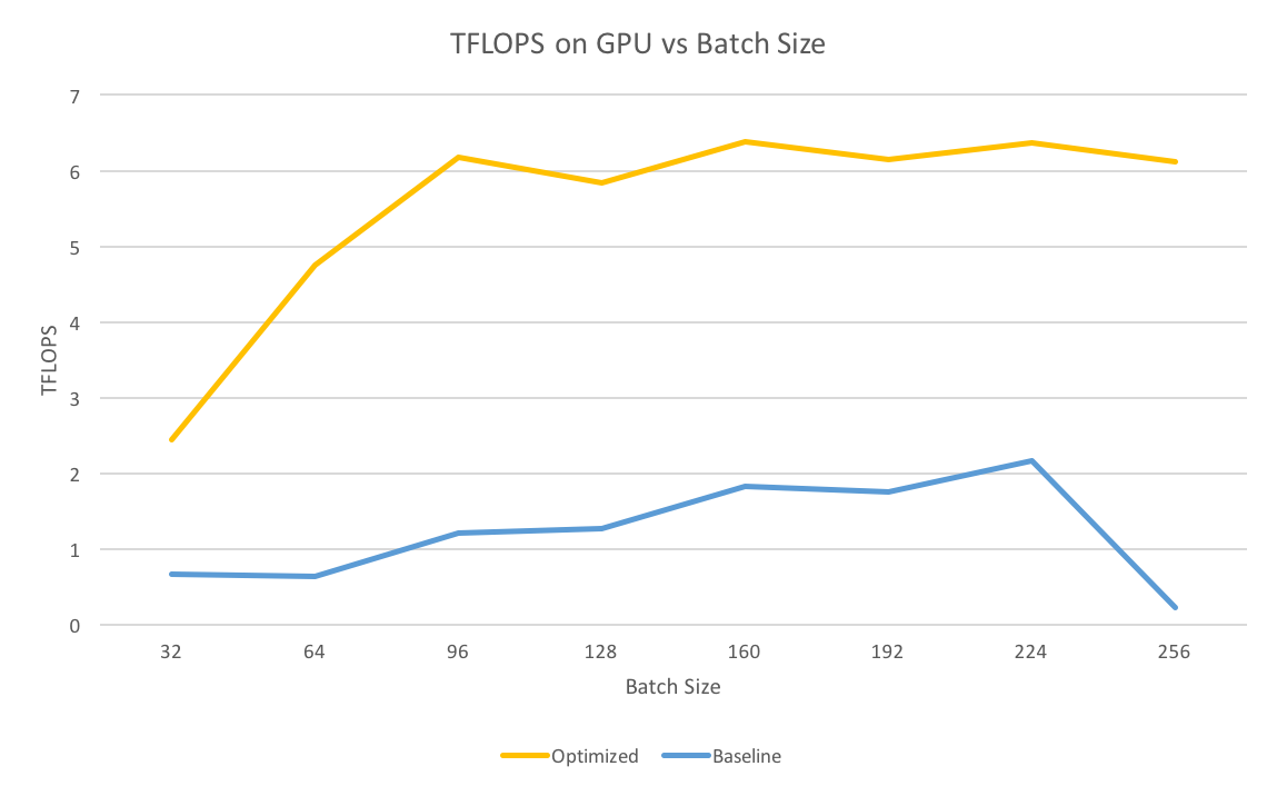 *Figure 5: Peak performance of GPU vs BatchSize.
Matrix Factorization
After our optimizations, we explored other algorithmic changes/approximations within LSTM cell that were possible to improve the performance further. One technique was to reduce the number of weights (parameters) within an LSTM cell. Figure 6 shows the computation within an LSTM cell.

*Figure 6: Matrix Factorization of LSTM
In this equations T is an affine transform $T = W * [x_t,h_{t-1}] + b$. The major part of the LSTM computation is spent in computing affine transform T as it involves the matrix multiplication with W which is of size 4n x 2p, where x and h are of dimension $n$ and i,f,o,g gates are of dimension $p$.
We can approximate W matrix as $W \approx W2 * W1$, where W1 is of size 2p x r and W2 is of size r x 4n. Note here we assume W can be approximated by a matrix of rank r.
Total number of parameters in W earlier: 2p * 4n
Total number of parameters in W after factorization: 2p * r + 4n * r
Computation time comparison for a LSTM configuration of hidden unit 256 and sequence length 100. Experiments were performed on Macbook Pro.
Standard LSTM : 42.8ms
Factorized LSTM : 8.36ms
Compiler Optimization for LSTM using XLA
Google recently launched a Just-in-Time compilation toolchain for TensorFlow called XLA. This is a Accelerated Linear Algebra tool chain which fuses multiple operations within the dataflow graph of TensorFlow and generates a in-memory binary using LLVM backend. Across iterations, the same binary is invoked to perform computations. We wanted to analyze the speedup and efficiency of XLA for LSTMs and we performed a few experiments on the same. On a Intel i5 1.6Ghz CPU, we saw significant improvement in performance with XLA. We experimented with an LSTM cell of size 1024 and compared the perfomance with XLA and without XLA. The Speedup achieved with XLA as the matrix size increases from 10 to 1024. This is mainly due to the the JIT compilation overhead for smaller matricies. As shown in Figure 6, XLA’s JIT compilation provides significant improvement for larger matricies.
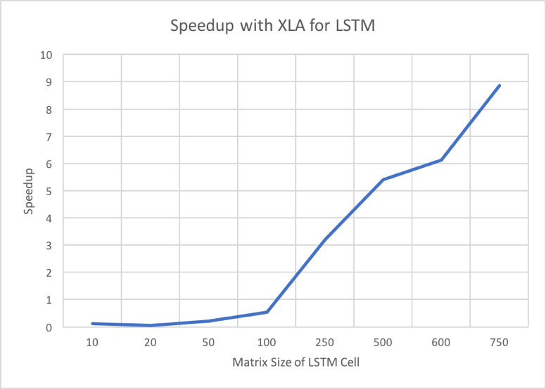
Figure 7: Speedup with XLA for LSTM vs Matrix Size.
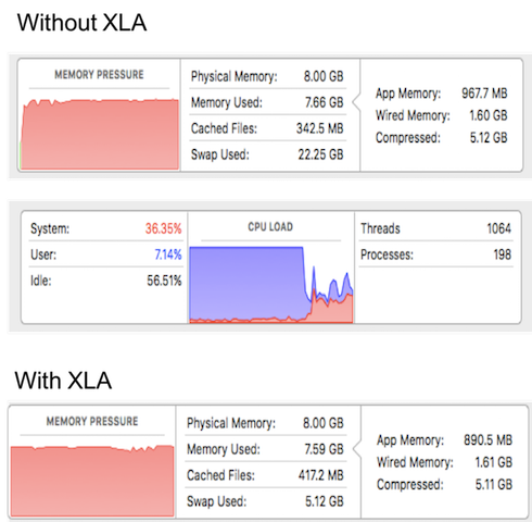
Figure 8: Memory consumption for LSTM cells with and without XLA.
One of the key optimizations that XLA performs is the elimination of intermediate buffers by fusing operations. As shown in Figure 7, the memory consumption without XLA is approximately 22.5GB and 5.12GB with XLA. Due to large memory requirements, the memory bandwidth requirement increases. Due to swapping and memory latency, the cpu spends most of the time waiting for the data. XLA clearly improves the performance in this aspect for LSTMs.
The Challenge
- Since this is our introduction to Domain Specifc Languages, we assume the learning curve would be steep and hence we plan to initially spend some time to understand the code structure in Halide.
- Training of LSTM’s using Backpropogation Through Time is a tricky process and might take time to get the gradient calculations right. We can initially try to optimize just for inference using pre-trained network and if the time permits, optimize for backpropogation.
Conclusion
In conclusion, we aimed to improve the performance of LSTM forward propogation on NVIDIA’s GTX1080 GPU. We optimized the baseline code mainly to utilize all the available GPU resources, exploit cache locality and reduce the number of kernel invocations. We also implemented a scheduling algorithm for LSTM cells to compute independent cells in parallel. Overall, we achieved a speedup of 7.98x.
Platform Choice
The GTX 1080 GPU’s on GHC.
References
- Optimizing Performance of Recurrent Neural Networks on GPUs Link : https://arxiv.org/abs/1604.01946
- https://devblogs.nvidia.com/parallelforall/ optimizing-recurrent-neural-networks-cudnn-5/
- http://svail.github.io/diff_graphs/
- http://svail.github.io/rnn_perf/